Clustering: Using the City of Toronto's Open Data to Analyze Councillor Voting Behaviour
Canadian municipal politics is arguably the most important form of politics to those who live in the jurisdiction, but it can also be impenetrable to outsiders due to the lack of parties, platforms, and the highly specific local issues that are debated. Could we determine which voting blocs exist without this information? Can we determine which politicians make compromises and which refuse to bend?
I wrote a clustering algorithm to group councillors based their voting records, developed it with Toronto data and evaluated it with Calgary data, and you can see the jupyter notebook here. This is, in a sense, a continuation of the analysis being done in my previous post.
For the technically-minded reader, the clustering algorithm was a heirarchichal agglomerative clustering using a Bayesian probability of the councillors within the group not being unanimous as the objective function to be minimized. Some analysis is done to identify how a binomial distribution can reasonably be applied to the data despite not having any knowledge of the issues being voted upon. Lastly, the Hartigan-Wong algorithm was applied to ensure we were at a (at least local) minimum.
Initial Exploratory Data Analysis
Overview
Many municipalities have open source data available on a very wide number of topics. For example, in Toronto you can find data on everything from all public city-provided wifi, to red-light camera locations, to restaurant food inspection results. Here are the data for Toronto and Calgary. Here I’ve used the data listing how councillors voted in all recorded city council meetings.
If we look at voting records we can try to group councillors together based on how similar they are from each other. To see if we’ve done a good job clustering, I built everything that follows using the Toronto council voting data. When I was satisfied that the results looked reasonable, I tested to see if it worked using the Calgary council voting data.
Unfortunately we see that there is a substantial difference between the two datasets. Toronto’s voting records go back to 2006, whereas Calgary’s only go back to 2017. To go back further with Calgary’s data, it looks like I’d have to do some pdf scraping of the meeting minutes. Since this is supposed to be a fun project, I’ll just let it be. If I were to do this again, I’d find a better train-validation-test breakdown.
Initial Exploratory Data Analysis
This is what our data looks like for Toronto:
| Term | First Name | Last Name | Committee | Date/Time | Agenda Item # | Agenda Item Title | Motion Type | Vote | Result | Vote Description |
|---|---|---|---|---|---|---|---|---|---|---|
| 2022-2026 | Paul | Ainslie | City Council | nan | 2023.FM1.8 | Election of the Speaker and Deputy Speaker | Nomination of a Member | Yes | Carried, 25-1 | Majority required - Appoint Councillor Nunziata as Speaker |
| 2022-2026 | Brad | Bradford | City Council | nan | 2023.FM1.8 | Election of the Speaker and Deputy Speaker | Nomination of a Member | Yes | Carried, 25-1 | Majority required - Appoint Councillor Nunziata as Speaker |
| 2022-2026 | Alejandra | Bravo | City Council | nan | 2023.FM1.8 | Election of the Speaker and Deputy Speaker | Nomination of a Member | Yes | Carried, 25-1 | Majority required - Appoint Councillor Nunziata as Speaker |
| 2022-2026 | Jon | Burnside | City Council | nan | 2023.FM1.8 | Election of the Speaker and Deputy Speaker | Nomination of a Member | Yes | Carried, 25-1 | Majority required - Appoint Councillor Nunziata as Speaker |
| 2022-2026 | Shelley | Carroll | City Council | nan | 2023.FM1.8 | Election of the Speaker and Deputy Speaker | Nomination of a Member | Yes | Carried, 25-1 | Majority required - Appoint Councillor Nunziata as Speaker |
And our data for Calgary:
| MeetingType | MeetingDate | Voter | Vote | Result |
|---|---|---|---|---|
| Audit Committee | 2022/01/20 | Lori Caltagirone | Yes | MOTION CARRIED |
| Audit Committee | 2022/01/20 | Karen Kim | Yes | MOTION CARRIED |
| Audit Committee | 2022/01/20 | John (Richard) Pootmans | Yes | MOTION CARRIED |
| Audit Committee | 2022/01/20 | Jennifer Wyness | Yes | MOTION CARRIED |
| Audit Committee | 2022/01/20 | Terry Wong | Yes | MOTION CARRIED |
In both tables, we have one entry per councillor/mayor and per motion. To cluster the councillors, we’ll want to identify each motion and then see how every councillor voted on that motion. We can do this with a pivot.
First though, we should understand the major features of the data. For example, almost all votes are Yes votes:
Toronto
| Vote | count |
|---|---|
| Yes | 507330 |
| Absent | 108378 |
| No | 91838 |
Calgary
| Vote | count |
|---|---|
| Yes | 25348 |
| No | 2897 |
| Absent | 10 |
When clustering councillors based on their votes, this propensity for Yes should be kept in mind!
One major difference between the datasets is apparent here… In Toronto absent councillors are always given a row in the data where they Vote Absent, whereas the absent councillors in Calgary are omitted from the table entirely, with rare exceptions.
In the Toronto data we have a feature called the Motion Type. I can imagine that some motions are controversial, some motions are skippable, and some are good reflections of a candidates viewpoints. Let’s see how it breaks down (sorted by proportion of No votes):
| Motion Type | Total | Yes % | No % | Absent % |
|---|---|---|---|---|
| Adjourn | 58 | 25.8621 | 56.8966 | 17.2414 |
| Amend Mayor’s Proposed Budget | 338 | 44.6746 | 54.7337 | 0.591716 |
| Amend Auditor General Workplan | 161 | 44.0994 | 44.0994 | 11.8012 |
| Amend Item (Two-Thirds) | 124 | 51.6129 | 42.7419 | 5.64516 |
| Receive Item | 7430 | 40.7402 | 38.6272 | 20.6326 |
| Set Committee Rule | 202 | 57.4257 | 33.1683 | 9.40594 |
| Refer Motion | 2447 | 55.3739 | 32.2844 | 12.3416 |
| Recess | 306 | 53.9216 | 31.0458 | 15.0327 |
| Meet in Closed Session | 10 | 60 | 30 | 10 |
| Amend Motion | 14162 | 59.349 | 29.9393 | 10.7118 |
| … | … | … | … | … |
| Adopt Order Paper as Amended | 4546 | 86.4936 | 0.945886 | 12.5605 |
| Petition Filed | 3394 | 84.4137 | 0.589275 | 14.9971 |
| Introduce Report | 3567 | 86.1789 | 0.476591 | 13.3445 |
| Adopt Minutes | 1823 | 80.2523 | 0.274273 | 19.4734 |
Here we reach a difficult decision… should any motion types be removed because they do not actually reflect councillor voting patterns, which is what we want to observe? You could argue that Adopt Minutes and Introduce Report are so agreeable that they offer little information about our voters, but it’s unclear how to define when a motion is meaningless compared to insightful. Even votes on banal-sounding issues like Recess could contain information on the political leanings of councillors, so it’s tough to justify removing any of these. Perhaps more importantly, it would be far more difficult to remove similar motions from the Calgary data since this information is obscured within the Resolution column, and treating the datasets differently would undermine comparisons between the two.
In light of this, I’ve chosen to keep all of our motion types. It’s something we can keep in mind if we ever revisit this analysis later.
So what’s the most commonly skipped motion? It’s Extend Speaking Time at almost 30%! My imagination paints an image of one councillor giving a long-winded speech, while the rest have fallen asleep and are unable to vote when the loquacious councillor wants more time to keep going!
Clustering Metrics
Pair-wise councillor similarity
Now we finally have our data in a format where we can compare how similar two councillors are based upon how frequently they vote together. More formally, we want to group councillors into $N$ clusters, and our choice as to which clusters get which councillors should minimize some sort of “internal cluster dissimilarity”, and this should ultimately somewhat agree with our intuition about how politics-savvy people already mentally group councillors. We also want to ensure we have clusters of “reasonable” size, so we probably don’t want situations where there is one big cluster and a dozen “clusters” with one councillor each.
Our councillors voting records are difficult to map into a low-dimensional space. We don’t just care how much they vote yes or no, since each motion could be very different from each other. Many clustering algorithms are centroid-based, and the concept of a centroid is difficult to define in this situation. (Perhaps you could make a $m$-dimensional centroid where $m$ is the number of motions, and the space is entirely binary, but I doubt this would work well). A pair-wise distance/dissimilarity matrix can be created based on how often councillors agree on a vote, but we have to keep in mind this matrix will be sparse when comparing councillors across different terms.
Since this is a fun project, let’s invent our own clustering algorithm, following some ideas given by the existing ones. To do this in a sensible way, we should make a model about how councillors vote.
One possible place to start is to assume that when some councillor $A$ gives a response on some motion $i$, it is essentially a Bernoulli trial with some probability $p_{Ai}$ of voting Yes and $1-p_{Ai}$ of voting No. Unfortunately we have no reason to suspect any relationship between $p_{Ai}$ and $p_{Aj}, j \neq i$. These probabilities would vary wildly motion to motion, so it’s difficult to make generalized statements about voting behaviour from this idea alone. For example, let’s pretend $A$ wants to develop more bike lanes. On a motion $i$ to turn on-street parking into a bike lane, $p_{Ai}$ is very high, but on a motion $j$ to remove a bike lane to allow construction vehicles to replace a water main, $p_{Aj}$ would be much lower.
However, when we look at two councillors, there is a different Bernoulli trial occurring… these two councillors will give the same response to a motion with some probability $p_{i}$ and different responses with $1-p_i$. We’ve seen that some motions are more likely to produce disagreements than others, but over a large enough sample size, it’s not unreasonable to say that these probabilities of (dis)agreement are fairly constant between those two councillors. In other words, we can assume $p_{i} = p_{j}, \forall i,j$. Suddenly, with a few caveats, we can arrive at a Binomial!
Specifically, if councillors $A$ and $B$ are both voting in $n_{AB}$ votes, they’ll agree $a_{AB}$ times with a probability of agreeing $A_{AB}$.
\[a_{AB} \sim \text{Binomial}(n_{AB},A_{AB})\]Before we get ahead of ourselves, what are those caveats?
- $A_{AB}$ is assumed to be independent of motion, which really only holds if each pair of councillors get a similar distribution of motions to vote upon and enough votes to let $A_{AB}$ truly represent some kind of average disagreement probability
- Councillors are assumed to be static and unchanging over the time they spend in office.
- Votes are assumed to be independent of one another.
There are more assumptions we could acknowledge, but these three seem the most dubious. If we ever wanted to return to this project and improve our confidence in the result, tackling caveat #1 by controlling the motion types represented in our data would be a good starting point!
From our data, $n_{AB}$ and $a_{AB}$ are numbers we can directly compute. $A_{AB}$ however needs to be estimated. We could simply use the maximum likelihood estimator (MLE):
\[\hat{A}_{AB} = \frac{a_{AB}}{n_{AB}}\]There are two issues with this. Firstly, not all estimates of $A_{AB}$ will be equal since some pairs of councillors will have thousands of votes and some will only have a few (represented by $n_{AB}$), and it would be good to differentiate these situations. Secondly, we will have some pairs of councillors that agreed every (or almost every) time they were able to vote together… this usually happens when $n_{AB}$ is very low, but that doesn’t mean we genuinely believe $A_{AB}$ should be one.
A bayesian approach tackles both these problems simultaneously. As is typical with estimating Binomial probabilities, we’ll use the Beta distribution as a conjugate prior for $A_{AB}$,
\[A_{AB} \sim \text{Beta}(\alpha,\beta)\]Now we’ve just pushed our problem onto estimating $\alpha$ and $\beta$. Bayesian inference gives us a means for updating our estimates for these two (hyper/meta)parameters as we acquire more data, specifically:
\[\alpha' = \alpha + a_{AB}\] \[\beta' = \beta + (n_{AB}-a_{AB})\]Which will then set our estimator to the following:
\[\hat{A}_{AB} = \frac{\alpha'}{\alpha'+\beta'}\] \[= \frac{a_{AB} + \alpha}{n_{AB} + \alpha + \beta}\]We need to know the values of $\alpha$ and $\beta$ before we have any data, this is known as our prior. We have several options here: we can choose the uniform prior of $\alpha = \beta = 1$ or perhaps the Jeffrey’s prior of $\alpha = \beta = \frac{1}{2}$. To help us decide, we have another problem that needs solving first.
How to cluster more than two councillors?
We can now find the relationship between two councillors, but how do we evaluate a set of several councillors? One possible way is to extend the idea of agreement to unanimity. The logic is the same, except that we count our binomial ‘successes’ as when every councillor in the group votes unanimously on the motion.
There are some problems with this:
- Unanimity becomes less likely when more councillors are added to a group, even if the $p_{i}$ is unchanged
- Sets with large numbers of councillors might suffer from such low instances of unanimity that we become quite sensitive to our priors.
- All non-unanimous motions are treated identically, even though a set of 10 councillors voting on a motion where only one disagreed should more strongly suggest a cluster than if 5 councillors vote each way.
There are other possible objective functions to use when clustering that do not have these difficulties, but they likely come with their own problems. I’ll discuss one in an appendix.
These three problems can be mitigated by looking at the particulars of our dataset. Problem 1 gives us a bias toward having clusters of equal size, which is arguably a good thing. Problem 2 is made less troublesome by the fact that our councillors are usually voting yes on every motion, so unanimity much more common than if they were voting yes and no equally. In addition, we likely want councillors who rarely had the opportunity to vote together to be clustered separately, since we intuitively wouldn’t see them as part of any sort of voting bloc. For example Rose Milczyn in Toronto was a councillor for a month and therefore we don’t mind if she gets a cluster all to herself.
Last, and most complicated, is problem 3. Here I’ll argue that we usually have enough unanimous votes to give us the insight that we need into the councillors, and it’s indicative enough of the similarity between groups. I recognize there are some other definitions of our objective functions we could use that could avoid this problem, but this is the simplest, and it still appears to work!
Can this help us choose a prior? Unfortunately non-informative priors cause us some difficulties due to the nature of the problem and our desired output. We want councillors to cluster based on their unanimity, but we want to bias groups of councillors who’ve rarely or never voted together from clustering. To do this, I found the best priors were ones that strongly assumed councillors would disagree, but were quickly overpowered when $n_{AB}$ grew. $\alpha = 0.25, \beta = 1.75$ seemed to work fine at keeping the larger dataset councillors grouping first before grouping new members. In layman’s terms, this is like assuming that every group of councillors has already voted twice together and agreed 1/4 of a time.
We finally arrive at an estimator,
\[\hat{A}_{AB} = \frac{a_{AB} + 0.25}{n_{AB} + 2}\]Implementing the clustering
We next compare every pair of councillors and determine how likely they are to agree, and form this into a similarity matrix.
Now we can begin clustering. To do this, we’ll use hierarchical, agglomerative clustering. First each councillor gets their own cluster, and we begin to merge pairs of clusters based upon maximizing the probability that the new cluster will be unanimous. We can do this in a brute-force method of checking each cluster pair and keeping track of the unanimity probability of the new cluster candidate that would occur if the cluster pair was merged. Thankfully we can save some time by only re-evaluating these new cluster candidates for pairs that include a newly-merged cluster.
We’ll keep track of the clusters as we merge them, along with their unanimity probability, which is our objective function. We merge until we have only two clusters remaining.
Now we have to answer the question: how many clusters is the most appropriate? To do this, we can use the ‘elbow’ method to determine the point where the objective function begins to rise rapidly as we continue to merge clusters. This point is a little arbitrary, but it should correspond to when merging clusters begins to cost more than the simplification of the model gained by merging. To find this point, I’ve plotted all the clusters and their objective function, and selected a value that seems to correspond to the ‘elbow’ by eye.
This is how the latest term of Toronto’s city council looks like as we clustered it:
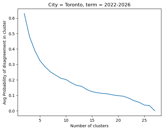
Looking at an elbow around 0.175 we have clusters that look like:
City = Toronto, term = 2022-2026
1 Anthony Perruzza
2 James Pasternak
3 Jaye Robinson
4 Lily Cheng
5 Mike Colle
6 Stephen Holyday
7 Amber Morley, Paula Fletcher
8 Dianne Saxe, Jamaal Myers, Olivia Chow, Chris Moise, Shelley Carroll
9 Josh Matlow, Gord Perks, Alejandra Bravo, Ausma Malik
10 Jon Burnside, Michael Thompson
11 Gary Crawford, Vincent Crisanti, Paul Ainslie, Nick Mantas, Frances Nunziata, Brad Bradford, Jennifer McKelvie, John Tory
That looks alright, though it’s not always good to see so many lonely clusters of single councillors. Can we do better? Yes, with Hartigan-Wong
Hartigan-Wong Method
An agglomerative clustering like this should work well when starting from an uninformed starting point to get us to a set of clusters that work okay, but the Hartigan-Wong method is the perfect way for pushing us from near a minimum to precisely finding that minimum. This method works by the following: we consider whether moving a councillor from one cluster to another reduces the objective function. If the answer is yes, then we do the move and repeat our search. In this implementation I made the first improving moves found, which is the fastest way to do this computationally. An alternative would be to search through all improving moves and make the move that improves the objective function the most. This best-move approach is more robust, but much slower. The first-move approach should be fine since we’re starting from what should be a relatively reliable clustering, so we’re unlikely to fall into any local minima.
The Final Clusters
Now that we’re happy all our councillors are where they belong, let’s try to visualize the new clusters. We can do this with a graph, where the distance between each councillor (the nodes) is influenced by the the pair-wise agreement matrix, and the colour of each councillor-node is coloured based on the cluster they ended up in. Note that our clusters care about group unanimity, which is a different thing from how often each pair of councillors agreed. This means that the position on the graph and the clusters shouldn’t agree perfectly, but should be close enough.
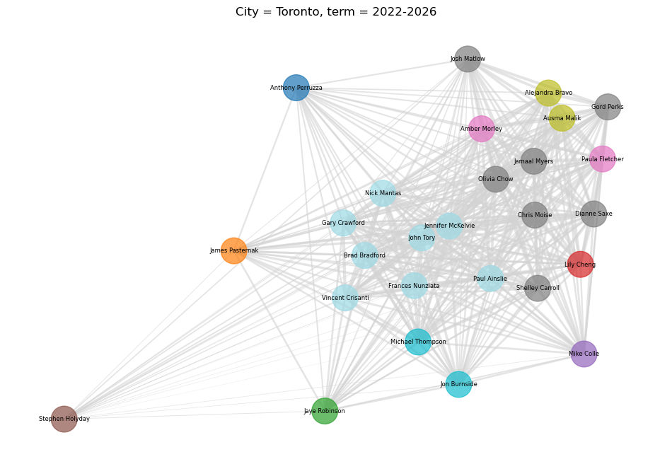
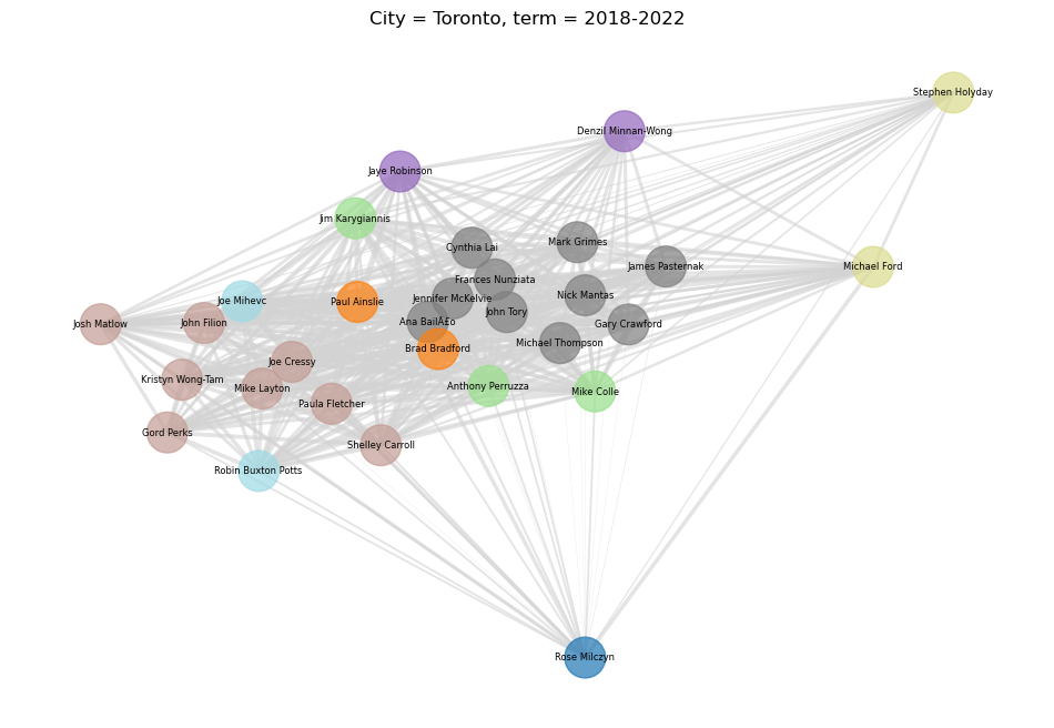
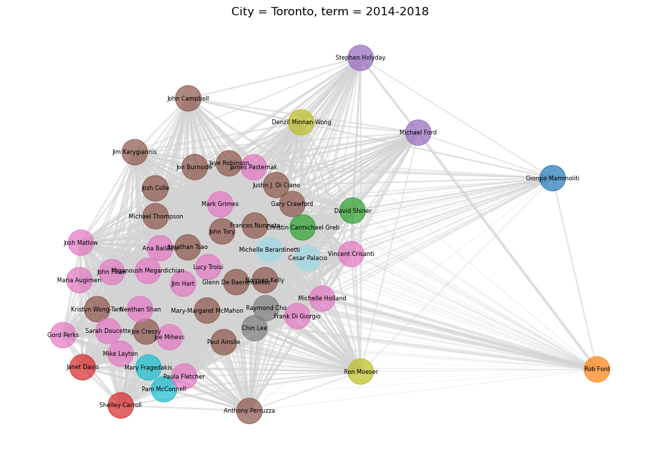
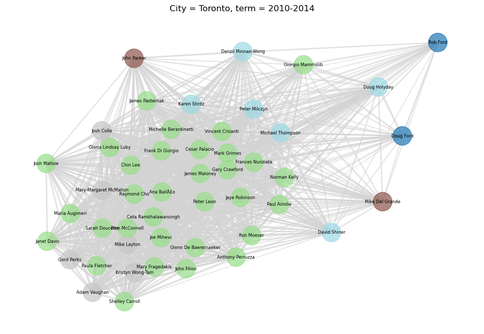
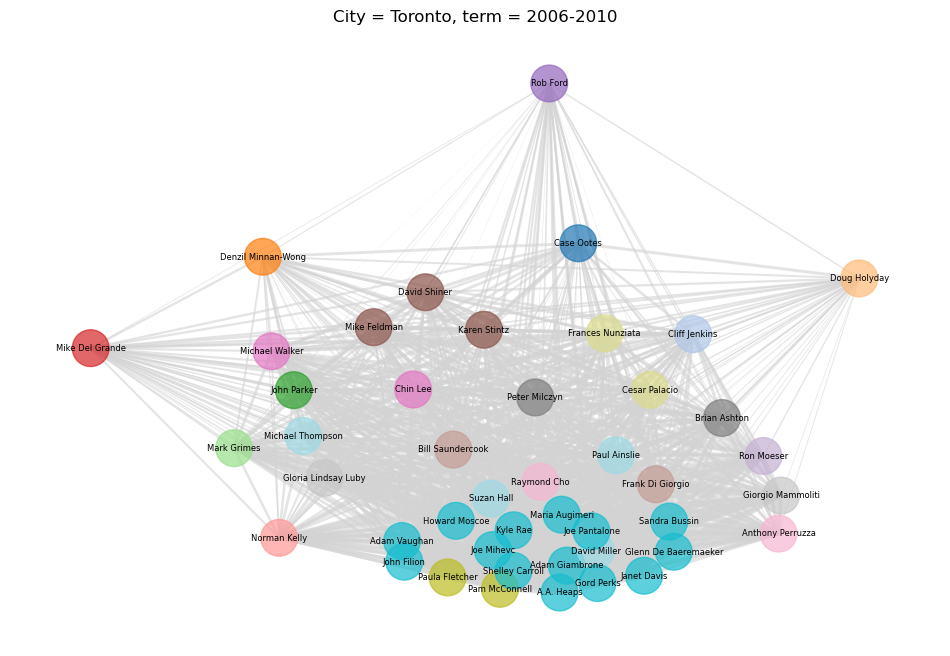
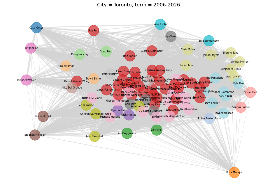
And if we try to cluster all Toronto councillors since 2006, we get the following:
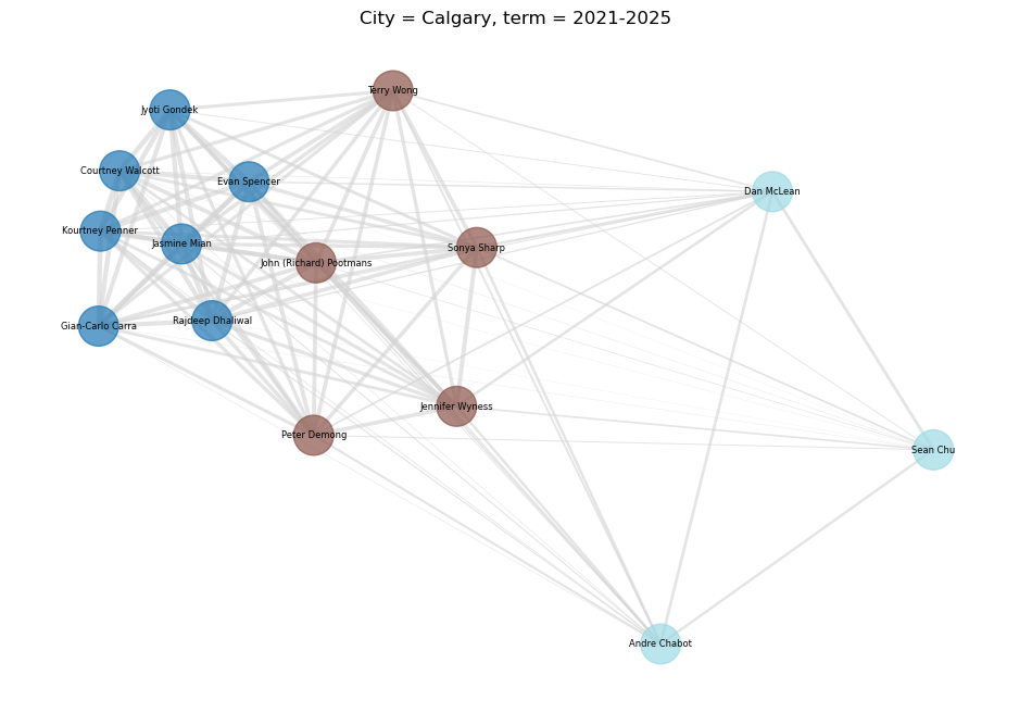
Looks good! Now for Calgary:

And both terms combined:
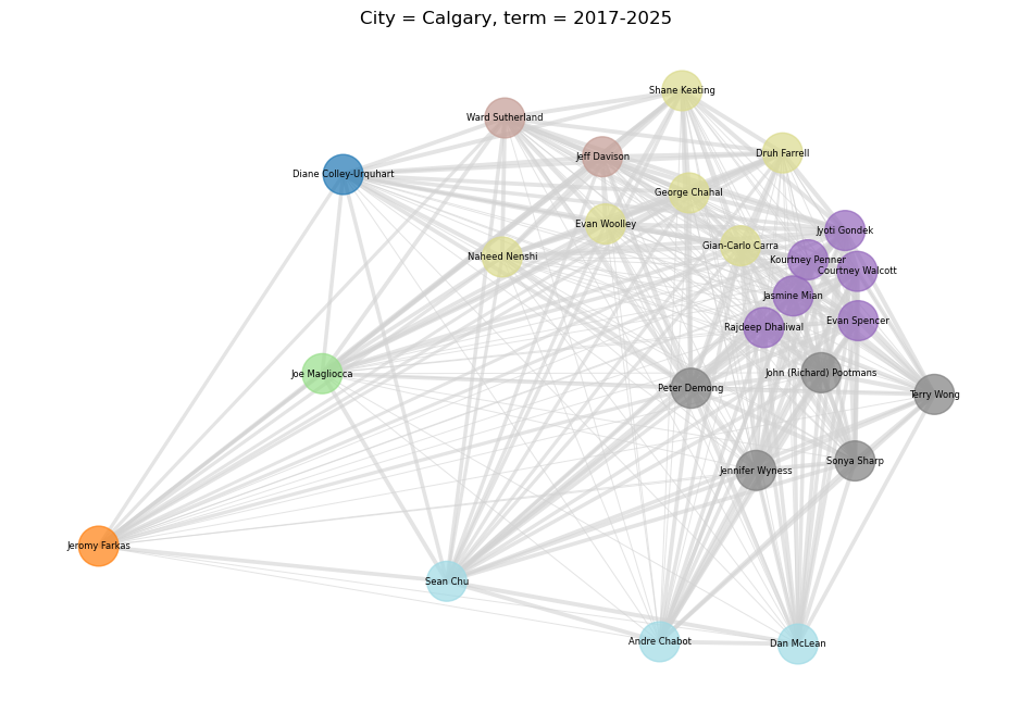
In general, this looks pretty good! I’m satisfied with the outcome. As we’d expect, the clustering is far more chaotic when there are multiple terms involved. The simple pair-wise agreement matrix, represented by the locations of the nodes, seems to work pretty well compared to the clustering, represented by the colour. It’s very apparent from this which councillors are likely to disagree frequently, as well as when we have common voting blocs.